Overview and Motivation
Various nonlinear control strategies are beneficial to deal with dynamic uncertainities of highly nonlinear, complex systems. One such system is the Iver3 Autonomous Underwater Vehicle(AUV). So during the second semester of my master’s I picked up this project along with another graduate student to test nonlinear control strategies for Iver3 AUV
The objective of the project is to generate a smooth trajectory to a desired goal position and to track the generated
trajectory using feedback control for an Iver3 AUV model. Seabed exploration is the practical scenario considered
to simulate the environment. Efforts were made to design a path planner that finds a smooth path in the presence
of obstacles and to design a controller that tracks the path found. The two different parts of the problem are
trajectory generation and trajectory tracking.
- Languages: MATLAB
- Skills : Nonlinear Control, Trajectory Generation, Trajectory Tracking, Path Planning
Approach
The model is an underactuated, nonlinear system. For the purpose of the project, a simplified 5-DOF model has been
considered. The AUV has three translational degrees of freedom in \((x,\ y,\ z)\) and two rotational degrees of freedom
in pitch \((\theta)\) and yaw \((\psi)\). The independent fins of the Iver3 model generate rotational motion whereas the thruster
produces surge velocity in the x-direction. The control inputs to the system are the normalized driving input \(\delta q\) ,
normalized rudder input \(\delta r\) , and the thruster rate \(\delta u\).
The dynamic model of the system has already been developed by the Dynamical Systems and Control Lab at JHU. One such model was used to test non linear control strategies for a trajectory generation and tracking problem. The states of the system are:
| Variables |
description |
| \((p_x,\ p_y,\ p_z)^{T}\) |
position vector |
| \(\theta\) |
pitch |
| \(\psi\) |
yaw |
| \(u_{v}\) |
surge velocity |
| \(q\) |
pitch acceleration |
| \(r\) |
yaw acceleration |
| \(T\) |
thrust force |
Trajectory generation
Differential Flatness
Differential flatness property can be quite useful to generate smooth trajectories for highly non linear systems. The flat output space that we chose for this system are \(y =\ (p_x,\ p_y,\ p_z)^{T}\) because we want the AUV to go from the initial position to a desired final 3D position. To prove that this is a flat for the nonlinear system, all the states and controls should be expressed as a function of the flat outputs and their derivatives.
\[\begin{matrix}
x & = & \phi(y,\ \dot{y},\ \ddot{y},\....,y_{(b)}) \\
u & = & \alpha(y,\ \dot{y},\ \ddot{y},\....,y_{(c)}) \\
\end{matrix}\]
Once thses conditions were checked, we generated the trajectory in flat output space using a polynomial basis function of the form \(\lambda(t)\ =\ (t^{5},\ t^{4},\ t^{3},\ t^{2},\ t,\ 1)^{T}\)
Trajectory Tracking
The equations for control inputs were solved using feedback linearization. The output states for this problem are \(y\ =\ (p_{x},\ p_{y},\ p_{z})^{T}\). With this in mind we can check if the system satisfies input-output linearization condition and have a control input that is of the form \(u\ =\ a(x)\ +\ b(x)v\) where \(v\ =\ y_{d}^{(3)}\ -\ k_{1}(y\ -\ y_{d})-k_{2}(\dot{y}\ -\ \dot{y_{d}})\ -\ k_{3}(\ddot{y}\ -\ \ddot{y_{d}})\) is the virtual input derived from the computed torque control law.
Modified RRT Path Planner
For a dynamic environment with obstacles, it is not ideal to generate trajectory at the beginning of the task. To address this issue, a RRT path planner was used to find a path from the intial position to the desired position. But when RRT find a new configuration from a current configuration, the current configuration is set as the initial configuration for the polynomial based trajectory generator and the next configuration is set as the desired configuration. If RRT find that this path is collision free, a smooth trajectory is generated using differential flatness based trajectory generation to avoid pointy path as in a typical RRT. These trajectory segments are stored and an overall trajectory is generated once the tree reaches the desired configuration. In order to target the goal, the algoroithm also has a random chance to attempt to reach the goal instead of choosing a random point.
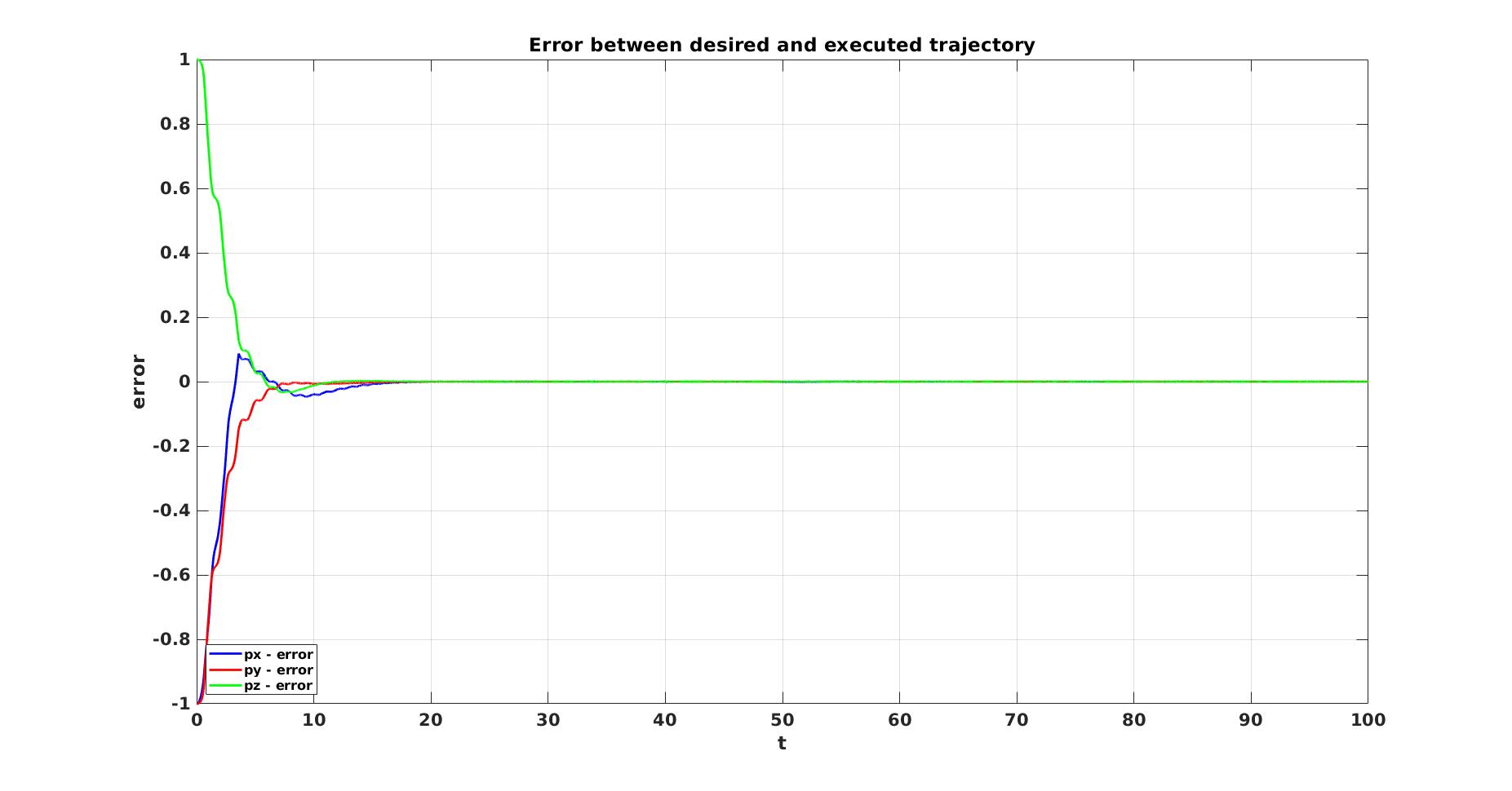
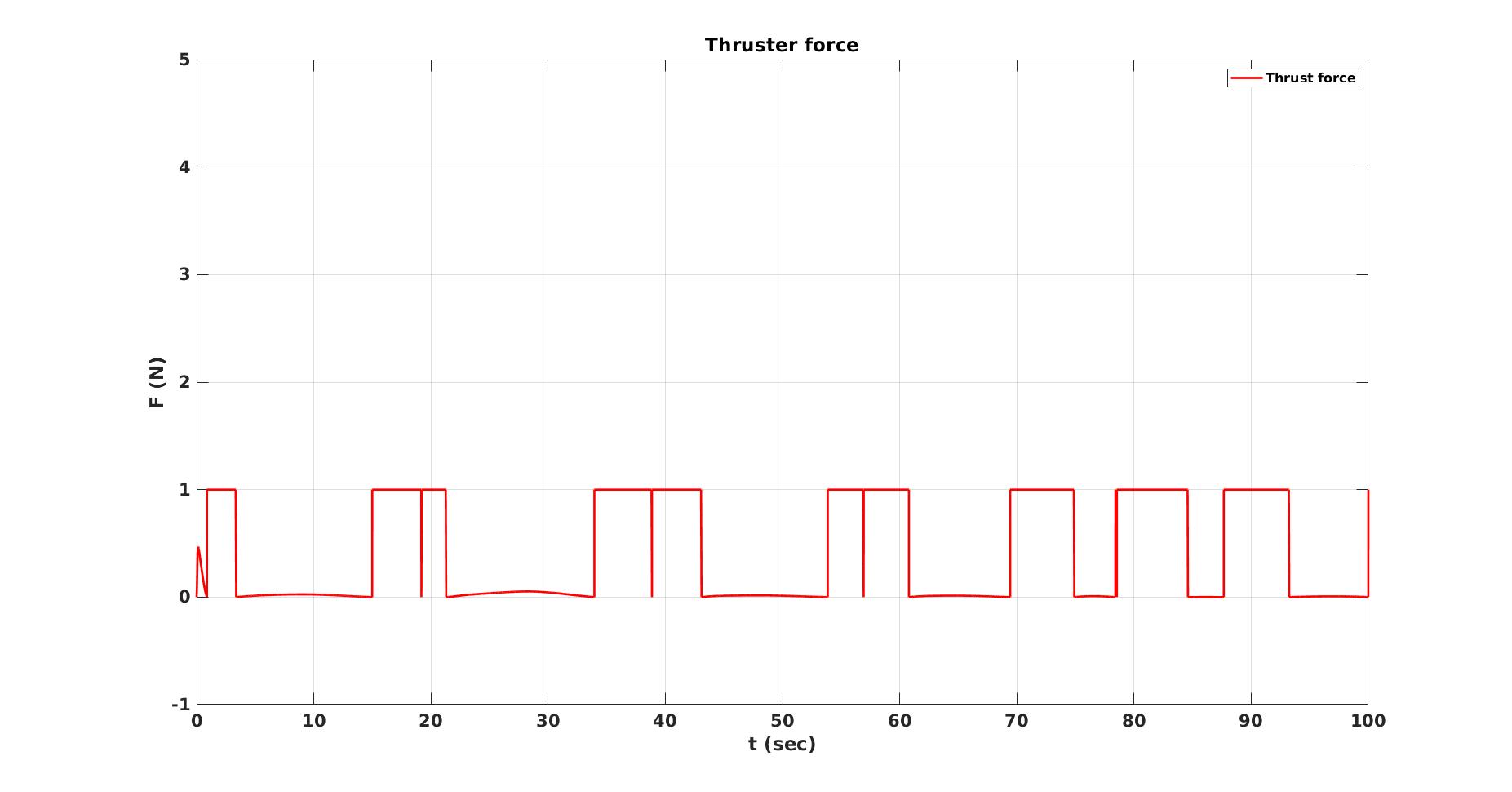
Result
Trajectory generation and tracking was done for three different initial conditions with perturbations for the 3D model of the system. The goal was for the system states \((y_1(t),\ y_2 (t),\ y_3(t))\) to follow \((y_{1d}(t),\ y_{2d}(t),\ y_{3d}(t))\). Here are the results for a slight perturbation in all degrees of freedom of the system.
| Errors in positio |
Thrust velocity for the system |
 |
 |
Challenges
- The solution does not consider constraints on the control and path. However, various optimization tools can be used for the same trajectory generation problem to include constraints and cost functional.
- The feedback linearization method might not be as robust as other nonlinear methods such as backstepping and lyapunov redesign.