Overview and Motivation
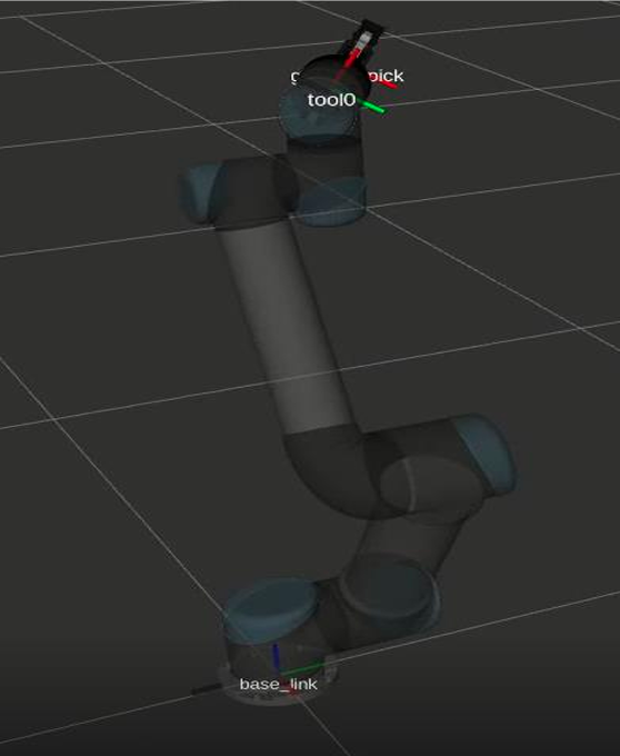
Move and Place is a very common industrial application of robotic arms. In my first semester in Robotics at JHU, I worked with two other graduate students to implement inverse kinematics solution for move and place application of UR5 arm.
- Languages: MATLAB
- Sottware : ROS
- Skills : Inverse Kinematics, Trajectory Generation
Approach
For a start and target location input,trajectory was planned using Inverse Kinematics Control,Resolved Rate Control and Transpose Jacobian Control.
For the inverse kinematics control, we designed a path by calculating a screw path from the starting position to the end position, and calculating frames along this path at specified intervals. Inverse kinematics was used to get the joint positions at each interval, which were then passed to the ur5_interface object to command the robot to each joint position.
The inverse kinematics problem deals with solving the equation \(g_{st}\ =\ g_{d}\) where \(g_{st}\) can be obtained from the forward kinematics map and \(g_d\) is the desired configuration. Both \(g_{st}\) and \(g_{d}\ \in\ SE(3)\). The problem might have a single solution, multiple solutions or no solution. A function was then written that gives 8 possible solutions of the generalized coordinates for any given homogeneous transformation. The algorithm followed to find the transformation required to move gradually from the start configuration to the final configuration is as follows:
- The initial and the final homogeneous transformations are decoupled into their respective rotation and translation part.
\(g_{initial}\ =\ (R_{initial},\ p_{initial}) \text{and}\ g_{final}\ =\ (R_{final},\ p_{final})\)
- A straight line path in the cartesian space is used to find the translation and rotation at any instant of time. Here the time interval considered is t[0,1], the increments are done in 0.1.
\(\begin{matrix}
p(t) & = & p_{initial}\ +\ t(p_{final}\ -\ p_{initial}) \\
R(t) & = & R_{initial}e^{(log(R_{initial} T R_{final})t)} \\
\end{matrix}\)
- So at t = 0, \(p(t)\ =\ p_{initial}\) , \(R(t)\ =\ R_{initial}\) and at t = 1, \(p(t)\ =\ p_{final}\) , \(R(t)\ =\ R_{final}\)
- The initial and final change as per the move and place function requirement.
- The \(g_{final}\) thus computed is used to find the possible solution to the inverse kinematics problem where \(\theta\ =\ f^{-1}(x)\) where \(f(x)\) is \(g_{final}g_{t}\). Here \(g_{t}\) is the transformation used to compensate the offset between the tool frame and the gripper frame.
- The solutions of the inverse kinematics are sent as an input to a function which checks for the best possible solution by considering each set of solutions as \(\theta\ =\ [theta_{1},\ theta_{2},\ theta_{3},\ theta_{4},\ theta_{5},\ theta_{6}]^T\)
- Based on the UR5 configuration, the observation that was made was that huge values of \(\theta_{1}\) and \(\theta_{2}\) increase the chances of collision with the table. - So any \(\theta_{1}\), \(\theta_{2}\) values that varied from the previous values of \(\theta_{1}\) and \(\theta_{2}\) by 30° were eliminated.
- Then the other values of the generalized coordinates were checked in a similar manner.
- These configurations were also checked for singularities at \(\theta_{3}\) and \(\theta_{5}\).
- Any configurations resulting in a homogeneous transformation that needs the gripper pick to collide with the table are changed to a cut off transformation in order to avoid collisions.
- The set of joint space coordinates that clears all these checks were used to move the robot in every iteration.
Rviz was used to visualize the control algorithm.
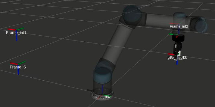
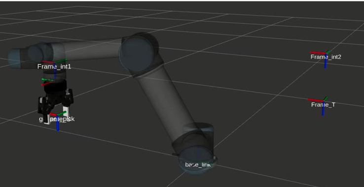
Result
| Moving to target location |
Moving back to start location |
 |
 |
Challenges
The solution proposed is not a robust way to check for singularities in joint angle solutions